Making Good Decisions given a Model of the World

Acting in a MDP

Recap:

$S$ -> State Space; $A$ -> Action Space
$s'$ -> $s_{t+1}$; $s$ -> $s_{t}$; and $s \in S$
Similarly, $a'$ -> $a_{t+1}$; $a$ -> $a_{t}$; and $a \in A$.
Note that, action $a$ is taken in current state $s$
Model: mathematical description of the dynamics and rewards of the agent’s including the transition probability $P(s' \mid s, a)$ (Probability of getting into new state $s'$ given, current state $s$ and action taken at this state $s$ is $a$)
Policy: function $\pi : S \rightarrow A$ => $\pi$ maps states to actions
Value Function: $V^{\pi}$ -> particular policy $\pi$ gives cumulative sum of future discounted rewards obtained by the agent.
$$V^{\pi}(s) = \mathbb{E}_{\pi} [r_{t} + \gamma r_{t+1} + \gamma^{2} r_{t+2}\hspace{2pt}+\hspace{2pt} ... \mid s_t = s]$$
Markov Property: Future is independent of past, given present

$$P(s_i \mid s_0, ..., s_{i−1}) = P(s_i \mid s_{i−1}), \forall \hspace{2pt} i = 1, 2, ...$$

Markov Process (=> Memoryless Stochastic Process)

Stochastic process satisfying Markov Property
Two assumptions:
- Finite State Space
- Stationary Transition Probability: Stationary => Time independent i.e. transition does not depend on time-step and only on states
Processes with these assumptions => Markov Chain
Such a transition matrix P is a Row Stochastic Matrix (means each element is non-negative (since all are probabilities $\in [0, 1]$) and sum of each row = 1)
$\textbf{s P} = \textbf{s'}$
$1 \times 6 \cdot 6 \times 6 = 1 \times 6$

Markov Reward Process

tuple of ($S, \textbf{P}, R, \gamma$)
Reward Function:
- Maps states to rewards (real number) => $R: S \rightarrow \mathbb{R}$
- Each transition $(s_i \rightarrow s_{i+1})$ is accompanied with a Reward $r_i$
- \[R(s) = \mathbb{E}[r_i \mid s_i = s]\]
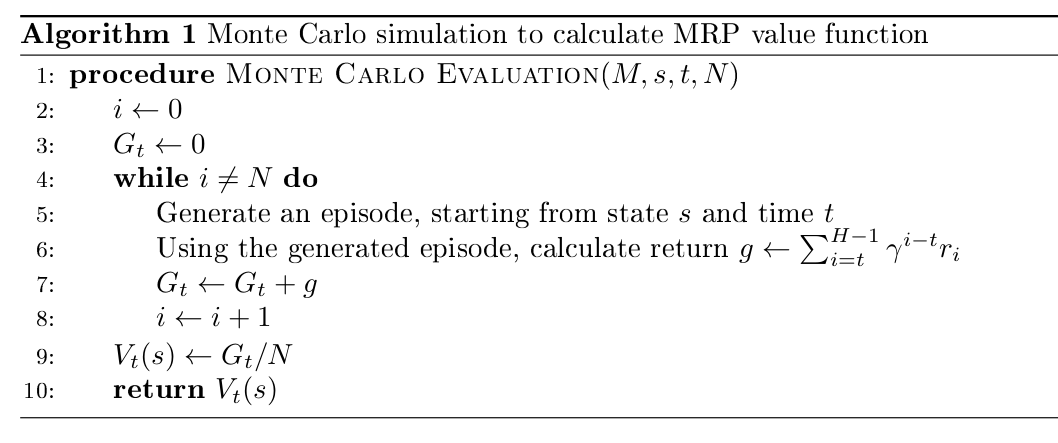
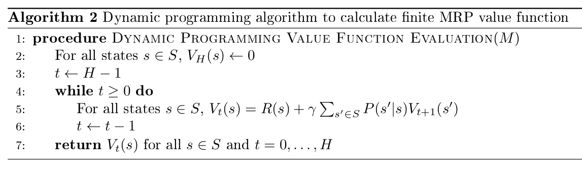
- Horizon: No. of time steps in each episode (can be infinite, else called finite Markov reward process)
- Return: Discounted sum of rewards from time t to horizon H
  $$ G_t = \sum^{H-1}_{i = t} \gamma^{i-t} r_i$$
- State Value Function: Expected return starting from state $s$ at time $t$
  $$V_t(s) = \mathbb{E} [G_t \mid s_t = s]$$
- In deterministic process, $G_t$ and $V_t(s)$ are identical. (Stochastic will be different)
Discount Factor ($\gamma$):
- We tend to put more importance in immediate rewards over the rewards obtained at a later time. Hence $\gamma \in [0, 1)$ is introduced.
  If $\gamma = 1$, and horizon $H \rightarrow \infty \Rightarrow V(s) \rightarrow \infty$.
- It is fairly accurate to have $\gamma = 1$, if $H$ is finite. But note that, $\gamma = 1$ denotes, all the rewards are equivalent in spite of the fact you reach the final state or not (You may consider a case, when an agent jumps to and fro between two states, infinitely).
- Geometric progression of $\gamma$ is the most efficient and effective way, currently*.

Calculation of State Value Function

Monte Carlo Method
- Generate episode -> Calculate Reward -> Average for each episode
Analytical Solution
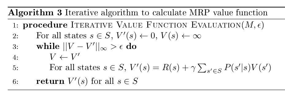
- Works only infinite horizon Markov Reward Process with $\gamma$ < 1.
- \[V(s) = R(s) + \gamma \cdot \sum_{s' \in S} P(s' \mid S) V(s')\]
- Vectorized Notation:
  
  $$V = R + \gamma \textbf{P}V$$
  $\textbf{P}$ is Probability Transition Matrix equivalent to $P(s' \mid S)$
- Above equation can be rearranged to
  $$(\textbf{I} - \gamma \textbf{P})V = R$$
  which has an analytical solution $$V = (\textbf{I} - \gamma \textbf{P})^{-1} R$$
- In above solution, note that, $\gamma < 1$, and $\textbf{P}$ is row stochastic, $(\textbf{I} - \gamma \textbf{P})$ is non-singular => it can be inverted. Thus, $V = (\textbf{I} - \gamma \textbf{P})^{-1} R$ always has a solution and the solution is unique.
Iterative Method
- Finite Horizon => *Dynamic Programming*
  - \[V_t(s) = R(s) + \gamma \cdot \sum_{s' \in S} P(s' \mid S) V_{t+1}(s') \hspace{8pt} \forall \hspace{3pt} t = 0, 1, ..., H - 1.\]
- Infinite Horizon => *Iterative*
Note:
- The computational cost for Algorithm 1 is $O(\mid S \mid ^3)$ where as for Algorithms 2 & 3 it has been improved to $O(\mid S \mid ^2)$. All of them converge to the correct solution as described by Theorem 3.1 in Original Lecture Notes.

Markov Decision Process

tuple of ($S, A, \textbf{P}, R, \gamma$)
Major difference from MRP, is the inclusion of Action space $A$:
- Now, the transition probability will be defined with the action $P(s_i = s' \mid s_{i-1} = s, a_{i-1} = a)$
- Similarly, reward is defined as
  $$R(s, a) = \mathbb{E}[r_i \mid s_{i} = s, a_{i} = a]$$
MDP Policy: $\pi (a \mid s) = P(a_t = a \mid s_t = s)$ can be deterministic or stochastic.
For generality: Consider it as conditional distribution.
MDP + $\pi(a \mid s)$ = Markov Reward Process (Think about it, if can’t find answer, look the printed notes)
- => MDP can be evaluated in a similar fashion to MRPs.

Bellman Backup Operator(s)

We know that, if there is a MDP $M = (S, A, \textbf{P}, R, \gamma)$ and a (deterministic/stochastic) policy $\pi (s|a)$, it can be considered equivalent to MRP $M' = (S, \textbf{P}, R, \gamma)$.

=> The value function of the policy $\pi$ evaluated on $M$, denoted by $V^\pi$, is actually same as value function evaluated on $M'$. $V^\pi$ lives in the finite dimensional Banach Space ($\mathbb{R}^{\mid S \mid}$).

Trivia: Banach Space $\mathbb{R}^{\mid S \mid}$ is a complete vector space with norm $\Vert .\Vert$. Normed Vector Space is basically a space where norm is defined ($x$ -> $\Vert x \Vert$) or intuitively, the notion of “length” is captured.

Then, for an element $U \in \mathbb{R}^{\mid S \mid}$, Bellman expectation backup operator is defined as

$$(B^\pi(s)) = R^\pi(s) + \gamma \sum_{s' \in S} P^\pi(s'|s) \cdot U(s'); \forall s\in S$$

This equation is also termed as Bellman Expectation Equation.

Similarly, for an element $U \in \mathbb{R}^{\mid S \mid}$, Bellman optimality backup operator is defined as

$$(B^\pi(s)) = \max_{a \in A} \Big [ R^\pi(s) + \gamma \sum_{s' \in S} P^\pi(s'|s) \cdot U(s')\Big]; \forall s \in S $$

This equation is also termed as Bellman Optimality Equation.

The $\max$ operation in Optimality Equation brings the non-linearity in $U$, due to which, there is no closed form solution as in the case of Expectation Equation. Ref: StackExchange

MDP Control

\[\pi^*(s) = \arg \max_{\pi} V^{\pi}(s)\]
There exists a unique optimal value function.
Optimal Policy (not unique, like optimal value function) for a MDP in an infinite horizon problem is deterministic.

Policy Iteration & Value Iteration

Taken from Stack Overflow

Policy iteration includes: policy evaluation + policy improvement, and the two are repeated iteratively until policy converges.
Value iteration includes: finding optimal value function + one policy extraction. There is no repeat of the two because once the value function is optimal, then the policy out of it should also be optimal (i.e. converged).
Finding optimal value function can also be seen as a combination of policy improvement (due to max) and truncated policy evaluation (the reassignment of $V(s)$ after just one sweep of all states regardless of convergence).
The algorithms for policy evaluation and finding optimal value function are highly similar except for a max operation.
Similarly, the key step to policy improvement and policy extraction are identical except the former involves a stability check.