Machine learning is a field of study which focuses on the improvement of the performance measure through experiences for some specific tasks. With the introduction of LeNet by Prof. LeCun on the classification of handwritten digits (MNIST) dataset in late 90s, people in research community came to an understanding that neural networks with more than one hidden layers can achieve state of the art (SoTA) results (which was a thought not much appreciated by researchers back then). The modern advances in deep learning methods are facilitated due to the presence of large amount of data and computational power provided through the GPUs and hence giving rise to huge networks like GPTs (GPT-3, being most recent), ResNet, VGG etc. In this article, we will be focusing on the foundational idea of Neural Networks on which these SoTA architectures are built upon.

Neurons

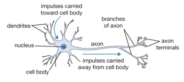
A brain, in general, harnesses the network of neurons to perform dozens of complex tasks efficiently. Every neuron processes signals entering from a dendrite and gives an output which is sent to the other neuron(s) and processed upon further. Hence, we can evidently state that removal of the network or even the reduction in the complexity of networks can harm its decision making process.

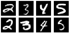
mnist_snap — A snapshot from MNIST Dataset.

The handwritten digits, for instance, are easily interpreted by the brain to differentiate between the digits, but if we have to write a program to classify them, it would be quite an arduous task. To solve this task, we take some inspiration from these dynamically activating neurons, and formulate a way to mimic it. The whole idea of Machine Learning and Artificial Intelligence is to develop a computer program comprising of artificial neurons (because, neurons are the most powerful entities to perform complex tasks) which shall eventually outperform the capabilities of a human brain.

The impulses from the sensory parts of the body reach the dendrite and if they are strong enough to create a stimulation, the axon outputs a spike. Since, biological neurons are living cells, they can modify themselves to define a stimulation threshold and hence are dynamic in nature.

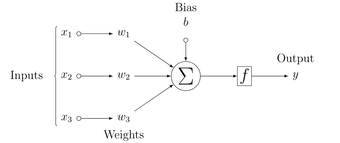
Similarly, the artificial neuron has some inputs and each of the input ($x_i$) is attached to a weight ($w_i$) and bias ($b$) (which are learned during their training period). The weight influences the importance of particular input. They perform a computation and produce a signal, which is forwarded through an activation function ($f$), to produce an output spike ($y$), given that such signal from $f$ is above the threshold value.

To illustrate, let’s consider the MNIST handwritten digits. Each digit is $28\times28$ px in size and each pixel has a grayscale value lying in the range of [0, 1] where 0 & 1 represent black and white respectively. The 2-D array is reshaped to a single dimensional array $x$ of length 784, and each index corresponds to an input pixel ($x_i$). We know that the black/dark pixels do not contribute to the curves/textures, hence they have less importance and light/white pixels exhibit quite significance in the determination of the digit (label). The relevance of a specific pixel (termed as a feature) is determined by the weights attached.

Single Layer Network

$$\begin{equation} y = f(\sum x_i\cdot w_i + b) \label{Eq:linearregression} \end{equation}$$

Eq. 1

Equation 1, mathematically, describes the basic functioning of a single layer network. It also establishes its relationship with a biological neuron. Precisely, the output $y$ is a function of an affine transformation of input features, characterized by a linear transformation of features via weighted sum, combined with a translation via the added bias.

The major goal of the single layer model lies in the identification of a set of weights ($w_i$) for corresponding input ($x_i$) so as to fit the data efficiently for our predicted output ($\hat{y}$). This will ensure a generalized behaviour over the dataset.

Ignoring the function $f$ for a while, we understand that

$$\begin{equation} \hat{y} = x_1 \cdot w_1 + x_2 \cdot w_2 + ... + x_d \cdot w_d + b \label{eq:expandedlr} \end{equation}$$

Eq. 2

where $d$ is total number of features from a input${^1}$, $w_i$ are the required weights. If we collect all the features into a vector $\textbf{x} \in \mathbb{R}^d$ and all our weights into another vector $\textbf{w} \in \mathbb{R}^d$, the Equation 2 can be simplified using a dot product:

$$\begin{equation} \hat{y} = \textbf{w}^T \textbf{x} + b \label{eq:compactoned} \end{equation}$$

Eq. 3

The $\textbf{x}$ in Equation 3 corresponds to features of a single data point. To express $\textbf{x}$ for all the inputs (in the dataset) in a $\mathbb{R}^{n \times d}$ dimensional space, we introduce a design matrix $\textbf{X} \in \mathbb{R}^{n \times d}$ where each row corresponds to an example and every column for a particular feature.

Hence, equation 3 can be rewritten for $n \times d$ dimensional space as:

$$\begin{equation} \hat{y} = \textbf{X}\cdot \textbf{w} + b \label{eq:compactnd} \end{equation}$$

Eq. 4

and the search for the best parameters weights vector $\textbf{w}$ and bias $b$ lies in the objective function (quality measure) and the procedure to update the parameters for the improvement in quality.

$\circ$ Fun Fact : The vectorized equations (such as in Eq. \ref{eq:compactnd}) simplify the math and make sure the code runs faster$^2$. In fact, a GPU has a lot more cores than a standard CPU (around 4000, in comparison to CPU’s 4 cores) and this allows the multi-threading processes to work efficiently, since computation in each cell of the matrix is independent of other cells.

Multi-layer Perceptron

As the name suggests, we, now, have more than one layer for our deep learning neural architecture. We described about the affine transformation (linear transformation with translation) in the previous section and described how an output from a single layered network is produced. In this section, we will dive deep into multi layer perceptron.

Hidden Layers

The linear models are based on a strong assumption that the a single affine transformation can map our input data to the outputs which is quite unrealistic. In addition, linearity implies monotonicity i.e. increase in the inputs eventually will either cause increase or decrease in the outputs. Let’s think about the classification of digits, the increase in intensity of a pixel doesn’t imply the increase in probability of getting a digit of higher magnitude. Hence, this assumption will surely fail in the case of image data (and of course, various other cases).

We have understood that the relevance of each input feature (pixel) is more complex$^3$ than expected. So, we introduce a few more fully connected (dense) layers between the inputs and output(s) which are termed as hidden layers. This architecture is referred to as Multi-layer Perceptron (MLP).

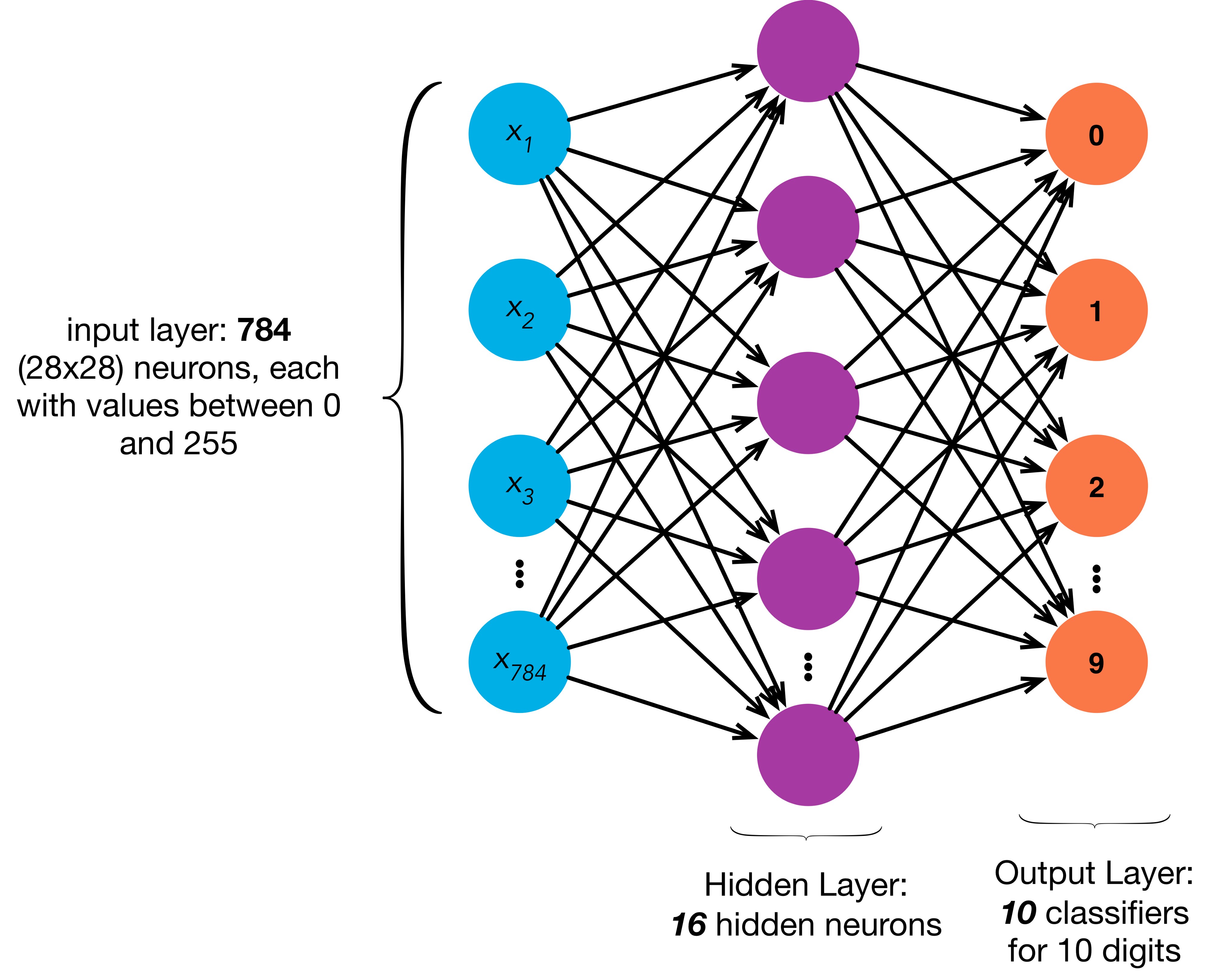
mlp — Illustration of Multi-layer Perceptron with a hidden layer of 16 neurons.

Taking up our classic example of MNIST Dataset, we will define a single hidden layer with 16 neurons as shown in Figure of MLP above. The figure lucidly explains the 784 input features, a hidden layer (more such fully-connected (dense) layers can be stacked, with any number of neurons), and output layer. Take a note that, neither input nor output layer is considered to be hidden.

Previously, we defined the input matrix as $\textbf{X} \in \mathbb{R}^{n \times d}$ where $n$ & $d$ are number of examples and features respectively. For a one-hidden-layer MLP, with $h$ neurons (hidden units), we can define a hidden layer matrix $\textbf{H} \in \mathbb{R}^{n \times h}$. Since the hidden and output layers are both fully connected, we have hidden-layer weights and biases as $\textbf{W}^{(1)} \in \mathbb{R}^{d \times h}$ and $\textbf{b}^{(1)} \in \mathbb{R}^{1 \times h}$ and output layer weights and biases as $\textbf{W}^{(2)} \in \mathbb{R}^{h \times c}$ and $\textbf{b}^{(2)} \in \mathbb{R}^{1 \times c}$. We have chosen simple (1) for first layer (the hidden layer) and (2) for second layer (the output layer) and $c$ is the number of classes. For our MNIST example: $n = 1, d = 784, h = 16, c = 10$.

Mathematically:

$$\begin{equation} \textbf{H} = \textbf{X}\cdot \textbf{W}^{(1)} + \textbf{b}^{(1)}, \textbf{O} = \textbf{H}\cdot \textbf{W}^{(2)} + \textbf{b}^{(2)} \label{eq:hoeq} \end{equation}$$

Eq. 5

which can be rewritten as

$$\begin{equation} \textbf{O} = (\textbf{X}\cdot \textbf{W}^{(1)} + \textbf{b}^{(1)}) \cdot \textbf{W}^{(2)} + \textbf{b}^{(2)} = \textbf{X}\cdot \textbf{W}^{(1)}\textbf{W}^{(2)} + \textbf{b}^{(1)}\textbf{W}^{(2)} + \textbf{b}^{(2)} = \textbf{X}\cdot \textbf{W} + \textbf{b}. \label{eq:hoopened} \end{equation}$$

Eq. 6

where $\textbf{W} = \textbf{W}^{(1)}\textbf{W}^{(2)}$ and $\textbf{b} = \textbf{b}^{(1)}\textbf{W}^{(2)} + \textbf{b}^{(2)}$.

The end result ($\textbf{O} = \textbf{X}\cdot \textbf{W} + \textbf{b}$) brings us back to a linear layer which practically equivalent to Equation 1. This means stacking linear layers over one another will again establish the linear behavior and will act as if only a single layer is present.

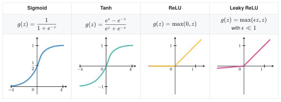
To inculcate a non-linear behaviour, each neuron in a hidden layer is subjected to an activation function $f$, and its outputs are referred to as activations. This activation function brings in a non-linearity and facilitates the MLP architecture to not fall back into a linear model. The equation 5 can be rewritten as: $\begin{equation} \textbf{H} = f(\textbf{X}\cdot \textbf{W}^{(1)} + \textbf{b}^{(1)}), \textbf{O} = \textbf{H}\cdot \textbf{W}^{(2)} + \textbf{b}^{(2)} \label{eq:hof} \end{equation}$

The activation function ($f$) brings up the required non-linearity, and hence, causes the stack of linear layers to be non-linear. This can be brought from various activation functions as shown in the given figure.

activationfxn — Commonly used non-linearities/activation functions ($$f$$).

This addition of non-linear layers increase the number of parameters in the neural network and hence, making it quite easy for the network to map any input with its output.

Conclusion

With above illustration and simple mathematics, we understood how Single Layer and Multi Layer Perceptrons function. We also looked into how GPUs facilitate the neural networks and how addition of non-linearity boosts the neural network architecture.

Footnotes

$^1$ $d$ is chosen (instead of an obvious choice $n$) due to the fact that all the features can be visualized in a $d-$dimensional space. $n$ is, however, used to denote the count of all the examples in a dataset.

$^2$ AI Stack Exchange Link: How do GPUs facilitate the training of a Deep Learning Architecture?